Fundamentals Of Statistics For Data Scientists and Analysts
Fundamentals Of Statistics For Data Scientists and Analysts ATTACH
Random Variables
a Random Variable is a way to map the outcomes of random processes, such as flipping a coin or rolling a dice, to numbers. For instance, we can define the random process of flipping a coin by random variable X which takes a value 1 if the outcome if heads and 0 if the outcome is tails.
we have a random process of flipping a coin where this experiment can produce two possible outcomes: {0,1}. This set of all possible outcomes is called the Sample Space of the experiment.
Each time the random process is repeated, it is referred to as an Event. In this example, flipping a coin and getting a tail as an outcome is an event. The chance or the likelihood of this event occurring with a particular outcome is called the probability of that event.
A Probability of an event is the likelihood that a random variable takes a specific value of x which can be described by P(x). In the example of flipping a coin, the likelihood of getting heads or tails is the same, that is 0.5 or 50%.
Mean, Variance, Standard Deviation ATTACH
The Population is the set of all observations (individuals, objects, events, or procedures) and is usually very large and diverse, whereas a Sample is a subset of observations from the population that ideally is a true representation of the population.
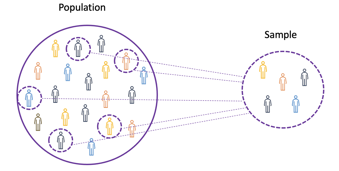
For this purpose, one can use statistical sampling techniques such as Random Sampling, Systematic Sampling, Clustered Sampling, Weighted Sampling, and Stratified Sampling.
Mean
Mean also known as the average, is a central value of a finite set of numbers.
Then the sample mean defined by μ, which is very often used to approximate the population mean, can be expressed as follows: \[ \mu = \frac{\sum_{i=1}^N {x_i}}{N} \]
The mean is also referred to as expectation which is often defined by E() or random variable with a bar on the top. For example, the expectation of random variables X and Y, that is E(X) and E(Y)
import numpy as np
import math
x = np.array([1,3,5,6])
mean_x = np.mean(x)
# in case the data contains Nan values
x_nan = np.array([1,3,5,6, math.nan])
mean_x_nan = np.nanmean(x_nan)
return mean_x, mean_x_nan
Variance
The Variance measures how far the data points are spread out from the average value, and is equal to the sum of squares of differences between the data values and the average (the mean). \[ \sigma^2 = \frac{\sum_{i=1}^N {(x_i - \mu)^2}}{N} \]
import numpy as np
import math
x = np.array([1,3,5,6])
variance_x = np.var(x)
# here you need to specify the degrees of freedom (df) max number of logically independent data points that have freedom to vary
x_nan = np.array([1,3,5,6, math.nan])
mean_x_nan = np.nanvar(x_nan, ddof = 1)
return variance_x, mean_x_nan
Standard Deviation
The Standard Deviation is simply the square root of the variance and measures the extent to which data varies from its mean. \[ \mu = \sqrt{\frac{\sum_{i=1}^N (x_i - \mu)^2}{N}} \]
import numpy as np
import math
x = np.array([1,3,5,6])
variance_x = np.std(x)

x_nan = np.array([1,3,5,6, math.nan])
mean_x_nan = np.nanstd(x_nan, ddof = 1)
return variance_x, mean_x_nan
Covariance
The Covariance is a measure of the joint variability of two random variables and describes the relationship between these two variables. It is defined as the expected value of the product of the two random variables’ deviations from their means.
import numpy as np
import math
x = np.array([1,3,5,6])
y = np.array([-2,-4,-5,-6])
#this will return the covariance matrix of x,y containing x_variance, y_variance on diagonal elements and covariance of x,y
cov_xy = np.cov(x,y)
return cov_xy
Correlation
The Correlation is also a measure for relationship and it measures both the strength and the direction of the linear relationship between two variables. \[ Cor(X,Z) = \frac{Cov(X,Z)}{\sigma_x, \sigma_z} \]
import numpy as np
import math
x = np.array([1,3,5,6])
y = np.array([-2,-4,-5,-6])

corr = np.corrcoef(x,y)
return corr
Probability Distribution Functions
A function that describes all the possible values, the sample space, and the corresponding probabilities that a random variable can take within a given range, bounded between the minimum and maximum possible values, is called a Probability Distribution Functions (pdf) or probability density. Every pdf needs to satisfy the following two criteria:
\begin{equation} \[0 \le Pr(X) \le 1\] \[\Sigma p(X) = 1\] \end{equation}
Probability functions are usually classified into two categories:
- Discrete Probability Distribution Discrete distribution function describes the random process with countable sample space, like in the case of an example of tossing a coin that has only two possible outcomes.
- Continuous Probability Distributions Continuous distribution function describes the random process with continuous sample space.
Binomial Distribution
The Binomial Distribution is the discrete probability distribution of the number of successes in a sequence of n independent experiments, each with the boolean-valued outcome: success (with probability p) or failure (with probability q = 1 − p). \[ f(k,n,p)=\Pr(X=k)={n \choose k}p^{k}(1-p)^{n-k} \]
Binomial Distribution Mean & Variance
\[ {E} [X]=np \] \[ {Var} [X]=np(1-p) \]
# Random Generation of 1000 independent Binomial samples
import numpy as np
n = 8
p = 0.16
N = 1000
X = np.random.binomial(n,p,N)

# Histogram of Binomial distribution
import matplotlib.pyplot as plt
counts, bins, ignored = plt.hist(X, 20, density = True, rwidth = 0.7, color = 'purple')
plt.title("Binomial distribution with p = 0.16 n = 8")
plt.xlabel("Number of successes")
plt.ylabel("Probability")
plt.savefig('assets/binomial-distribution.png')
return 'assets/binomial-distribution.png'
#+ATTR_ORG : :width 480
Poisson Distribution
The Poisson Distribution is the discrete probability distribution of the number of events occurring in a specified time period, given the average number of times the event occurs over that time period.
Poisson Distribution Mean & Variance
# Random Generation of 1000 independent Poisson samples
import numpy as np
lambda_ = 7
N = 1000
X = np.random.poisson(lambda_,N)

# Histogram of Poisson distribution
import matplotlib.pyplot as plt
counts, bins, ignored = plt.hist(X, 50, density = True, color = 'purple')
plt.title("Randomly generating from Poisson Distribution with lambda = 7")
plt.xlabel("Number of visitors")
plt.ylabel("Probability")
plt.savefig("assets/poisson-distribution-sample.png")
return "assets/poisson-distribution-sample.png"
Normal Distribution
The Normal Distribution is the continuous probability distribution for a real-valued random variable.
Normal Distribution Mean & Variance
# Random Generation of 1000 independent Normal samples
import numpy as np
mu = 0
sigma = 1
N = 1000
X = np.random.normal(mu,sigma,N)

# Population distribution
from scipy.stats import norm
x_values = np.arange(-5,5,0.01)
y_values = norm.pdf(x_values)#Sample histogram with Population distribution
import matplotlib.pyplot as plt
counts, bins, ignored = plt.hist(X, 30, density = True,color = 'purple',label = 'Sampling Distribution')
plt.plot(x_values,y_values, color = 'y',linewidth = 2.5,label = 'Population Distribution')
plt.title("Randomly generating 1000 obs from Normal distribution mu = 0 sigma = 1")
plt.ylabel("Probability")
plt.legend()
plt.savefig("assets/normal-distribution-sample.png")
return "assets/normal-distribution-sample.png"